
Insights · ArticleAI-Based Root Cause Analysis in Manufacturing: From Mere Suspicion to the True Cause
Alarm in Seconds, Root Cause Search in Weeks: Why Classic Root Cause Analysis Is Too Slow
On a connected production line, statistical process control (SPC) works like a highly sensitive smoke detector: it goes off as soon as a value drifts out of range. Digital control charts reliably show that something is burning. Where exactly the fire started and why remains unclear.
The real work only begins afterward: root cause analysis. In practice, it often takes days or even weeks. Cross-functional teams laboriously gather data from MES, historian, LIMS, ERP and maintenance systems, form hypotheses and work through them one by one. The problem: they usually only investigate what they already suspect.
Tools for automated root cause analysis promise to shorten this lengthy step considerably. This article looks at how such methods typically work, where they reach their methodological limits, and what decisive difference object-centric data modeling combined with causal methods can make.
The Classic Five-Step Process and Its Blind Spots
Most modern analysis approaches follow a standardized sequence:
- Detect the signal: An SPC alarm, outliers in optical inspection or declining process capability (a falling Cpk, the process capability index) trigger the analysis.
- Define the time window: The relevant observation window before the signal is set, matched to the cycle times and processing steps of the line.
- Collect variables: All available process variables are gathered (e.g., temperatures, pressures, torques, tool IDs, material components, shifts).
- Evaluate relationships: Each variable is tested mathematically against the quality characteristic, for example with correlation coefficients (continuous), chi-squared tests (categorical) or SHAP values.
- Output a ranking: The system delivers a list of conspicuous variables, sorted by strength, for the quality team.
Looking at all variables at once is real progress compared with a manual search. Still, the classic method suffers from three central weaknesses:
- Spurious correlations: A highly ranked variable is often only a side effect or consequence, not the actual cause of the defect.
- Hidden confounders: If a new material delivery and a particular shift coincide in time, both correlate with the defect. A simple ranking cannot separate these effects.
- Blind spots for combinations: Pairwise tests miss defects that only arise from the interplay of several conditions that are inconspicuous on their own.
Automated tools therefore do not deliver proof per se, but statistically grounded hypotheses. How precise these hypotheses are is decided long before the algorithm runs: in data preparation.
The Bottleneck: Flat Tables as a Dead End
Production data is fragmented by nature: process values recorded every second (historian), order data (MES), material master data (ERP), maintenance events (maintenance systems) and test results (LIMS).
Classic analysis methods, however, require a flat data table with exactly one row per case. This forces companies to link and heavily condense data in advance (e.g., into averages per part or the last value before an event).
Each of these condensations is an irreversible decision made up front. Anyone who boils tool temperatures down to an average will miss short, critical force or heat peaks during the joining process. The choice of features therefore determines in advance which causes the system can find at all. This brings back, through the back door, exactly the dependence on hypotheses that automation was supposed to eliminate.
The Object-Oriented View of Data: The Workpiece in Focus
A modern alternative does without rigid up-front condensation. Instead, all data is organized flexibly around the real object of analysis in discrete manufacturing: the produced part.
Xplain Data implements this approach with its patented ObjectAnalytics™ technology. Each physical part is modeled as a digital object that fully retains its original data structure:
- The operations it has passed through, including precise timestamps, machine and nest or tool ID
- The high-resolution original process curves (e.g., torque curves) during processing
- Assigned components, including their quality values from incoming inspection
- Exact maintenance and calibration histories of the machines involved
The decisive advantage: complex features (such as “tool was already above the critical cycle count in the second operation” or “last calibration was more than ten days ago”) do not have to be defined in advance. They are derived dynamically from the object during the analysis. The search starts without preconceived assumptions: the entire object is screened flexibly for relevant factors and time relationships.
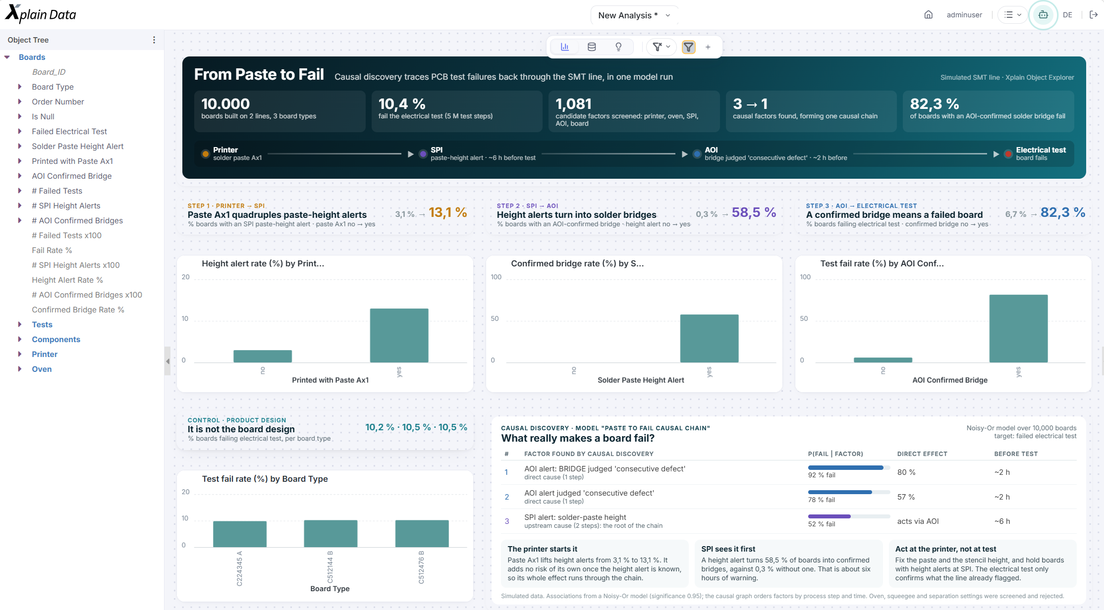
From Mere Suspicion to Causality: Isolating Confounders
To separate spurious relationships from true causes, causal methods check whether a statistical relationship remains stable when other influencing factors are controlled for.
A classic example from practice illustrates the confounder problem:
- Scrap occurs more frequently on the night shift.
- On the night shift, mainly material from Supplier B is processed, because its deliveries arrive in the evening.
- A standard pairwise test promptly flags both factors as highly suspicious.
If shift and material component are considered together, however, the shift effect disappears statistically. The material is the true cause; the shift is only correlated with the defect because both are linked to the material. For practice, this insight is business-critical: costly training for the night shift would have had no effect at all.
The CausalDiscoverer from Xplain Data builds directly on the object-centric data foundation (ObjectAnalytics). It isolates true drivers from mere spurious correlations and, instead of a one-dimensional list of variables, delivers a transparent network of causal dependencies.
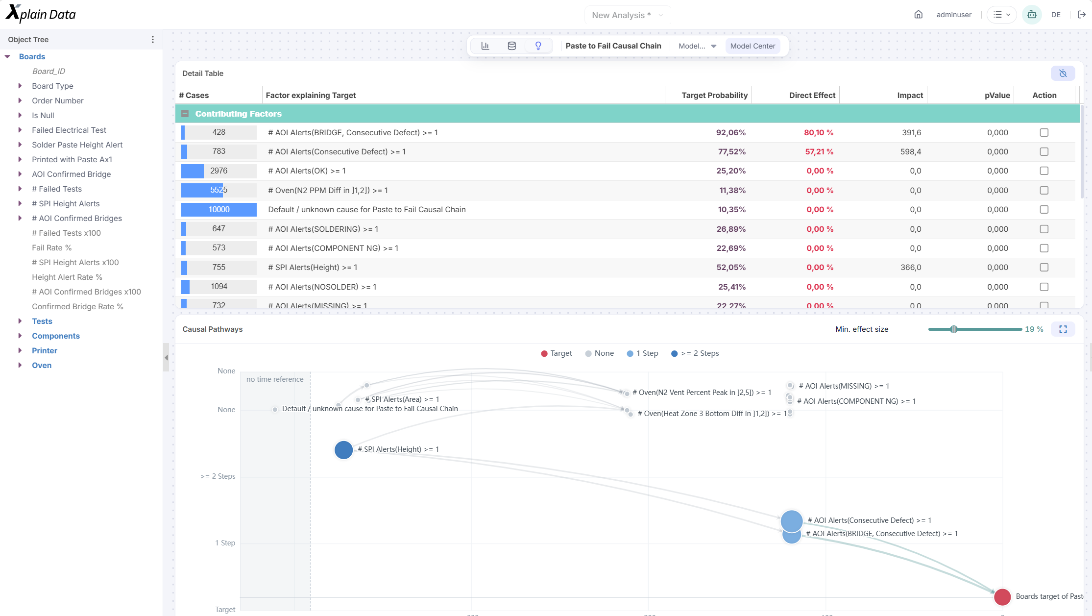
In Practice: Scrap Analysis on a Machining Line
On a precision line, the scrap rate in the final test creeps up over several weeks. The classic SPC charts do not trigger, because all individual parameters stay within their tolerance limits. A simple correlation analysis only shows vague, weak signals for shift, Machine 3 and Supplier B.
With object-centric modeling of each part, the automated causal search reveals the following picture:
| Factor | Pairwise view (classic) | Causal view (all factors considered) |
|---|---|---|
| Night shift | Conspicuous | No independent effect (spurious correlation) |
| Supplier B | Conspicuous | No independent effect (spurious correlation) |
| Machine 3 | Slightly conspicuous | Relevant only in one specific combination |
| Tool beyond service-life limit AND component with increased hardness | Not tested (invisible in a flat table) | Clear causal effect |
The critical combined feature in the last row did not exist in any source table. It only emerged from dynamically linking the exact tool condition with the hardness values of the material component at the exact time of processing.
Supplier B and the night shift appeared faulty in the standard analysis only because the harder raw material happened to be processed there. The resulting measure is now clear: the tool’s service-life limits must be shortened dynamically whenever harder material is used.
Where Automation Reaches Its Limits
No algorithm in the world can find causes that are not captured digitally. A reliable automated analysis stands or falls with five pillars:
- Complete traceability: Each part must be clearly linked to its operations, machines and installed components.
- Consistent timestamps: The clocks of process, maintenance and inspection systems must be synchronized so that time relationships can be reconstructed exactly.
- Sufficient data: To separate rare defect combinations cleanly from chance, a sufficient number of cases is required.
- Domain knowledge: Results from AI-based systems must never be adopted unchecked. Process experts must always check the statistical hypotheses for technical plausibility.
- Hidden variables: Unmeasured environmental influences (such as hall temperature or humidity) can still act as invisible confounders.
Automated systems therefore replace neither proven SPC charts nor structured problem-solving methods such as Ishikawa, 5-Why or 8D reports. Instead, they close the critical gap in between: they drastically shorten the path from the first workpiece alarm to a well-founded, testable hypothesis.
The great advantage of a system that monitors production automatically and continuously (through the Causal DiscoveryBot, an add-on to the CausalDiscoverer) is that problems do not first have to become so frequent or so severe that they hold up the entire production process, only to then require finding the actual cause with great effort and under time pressure. Typically, that is the moment when the relevant data, events and experts are brought together for targeted analyses. This is not only inefficient, it can also hurt on-time delivery.
In an automated data model, by contrast, where new data is loaded regularly (weekly, daily, hourly, …), the data can be examined for changes just as regularly and immediately. Alerts can be raised at the first suspicion, so that it can be checked as quickly as possible and the scenarios described above can be avoided.
Conclusion: Objective Hypotheses Instead of Human Assumptions
Automated root cause analysis significantly reduces the response time between defect detection and the final corrective action in discrete manufacturing. The quality of the results is determined less by the chosen algorithm than by the underlying data structure and the mathematical handling of confounders.
Classic tools that rely on pre-condensed, flat tables merely replicate the human hypotheses behind feature selection. Object-centric data management (with ObjectAnalytics), on the other hand, keeps the full level of detail of the discrete manufacturing steps flexibly available. Building on this, causal methods (CausalDiscoverer) separate true process drivers from mere statistical noise. The result is a data-driven, objective hypothesis, free of human preconceptions.
Frequently Asked Questions About AI-Based Root Cause Analysis
What is root cause analysis in manufacturing?
Root cause analysis looks for the actual cause of a quality problem, such as rising scrap or dimensional deviations. It usually starts when statistical process control (SPC) reports a deviation. The goal is a measure that fixes the problem permanently, not just the symptom.
Why isn’t SPC alone enough?
SPC reliably shows that a process has changed. It does not show why it has changed. In addition, control charts usually monitor individual parameters. Problems that only arise from the interplay of several inconspicuous variables therefore often go undetected.
What is the difference between correlation and causation?
A correlation only means that two variables occur together. Causation means that one variable actually influences the other. In manufacturing, the difference is decisive: a measure aimed at a merely correlated factor has no effect.
What is a confounder?
A confounder is a factor that influences two other variables at the same time and thereby creates a spurious relationship between them. An example: if a certain material is mainly processed on the night shift, the night shift can appear defect-prone even though the material is the cause. Causal methods take such factors into account; simple correlation rankings do not.
What data does automated root cause analysis need?
Traceability is key: each part must be linked to its operations, machines, tools and materials. Consistent timestamps from systems such as MES, historian, ERP, maintenance and inspection are also needed. In addition, there must be enough cases to distinguish real patterns from chance.
Does AI-based root cause analysis replace methods such as Ishikawa, 5-Why or 8D?
No. It complements these methods by shortening the path from a detected deviation to a well-founded hypothesis. Process experts still evaluate the result for technical plausibility, and any measure is confirmed in the process.
How do ObjectAnalytics and the CausalDiscoverer work together?
ObjectAnalytics brings all data from every production step for a part together in one object and preserves its original structure. This creates a complete view of the produced part. The CausalDiscoverer builds on this: it searches the object for influencing factors without prior assumptions (no feature engineering required) and separates true causes from spurious relationships.